Credit Risk Modelling

Disclaimer: The Process and the Charts are to be used carefully, as they change a lot based on the loan product type, customer cohort and other loan parameters. Here we have just presented a very generic overview of a vanilla product. All the data used for the credit risk modelling is with Roopya.

We explore the models created for the Roopya Score which aims to determine whether a customer’s creditworthiness is ‘Good’ or ‘Bad’ based on various input factors. We use various statistical methods used in credit scoring and provide an in-depth look at how the model was developed, including important considerations in the process. We also apply quantitative criteria to find the best model, highlighting its key qualities as an effective scorecard.

Start Free Trial

Using data from loan applications, we guide you through essential steps, including data preparation, selecting important features, converting variables using the Weight of Evidence (WOE) method, building the logistic regression model, conducting thorough evaluations, and ultimately creating a credit scoring system.

A credit score is a numerical representation of a customer’s creditworthiness. There are two main categories of credit scoring models: application scoring and behavioural scoring. Application scoring is used to evaluate the risk of default when a customer applies for credit, using data like demographic information and credit bureau records. Behavioural scoring, on the other hand, assesses the risk associated with existing customers. This is done by examining their recent account transactions, current financial data, repayment history, any delinquencies, credit bureau information, and their overall relationship with the bank. Identifying high-risk clients enables the bank to take proactive measures to protect itself from potential future losses.

Its Starts With Logistic Regression

Logistic regression stands as a fundamental technique frequently employed in the development of scorecards. This method comes into play when the predicted variable assumes a categorical nature. In instances where the predicted variable takes on a continuous form, linear regression takes the reins. In this section, we will delve into the application of multiple logistic regression for predicting binary outcomes, typically categorized as ‘good’ or ‘bad’.

Logistic regression, much like various other predictive modelling methods, leverages a set of predictor characteristics to gauge the likelihood or probability of a specific outcome—our target. The equation representing the logit transformation of the event’s probability can be articulated as follows:
Logit (pi) = 0 + 1×1 + 2×2 + … + kxk

Here’s a breakdown of the terms:

pi: The posterior probability of the event transpiring, given the input variables.
x: The input variables under consideration.
0: The intercept of the regression line.
k: Parameters associated with each input variable.

Evaluation Metrics

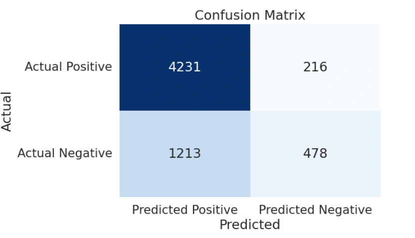
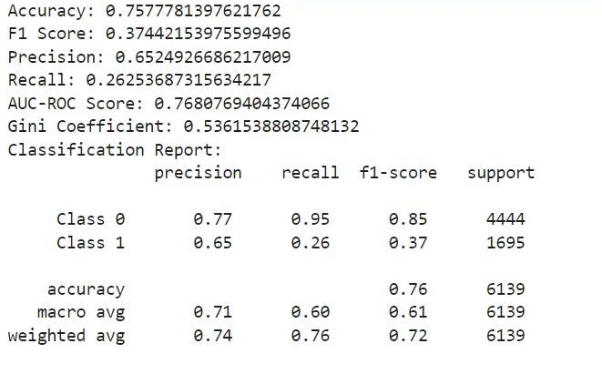
Several evaluation metrics are calculated to assess the model’s performance, including:

Accuracy
F1 Score
Precision
Recall
ROC-AUC Score
The Receiver Operating Characteristic (ROC) curve is generated to visualize models good bad classification power.
A classification report provides detailed metrics for both classes (Class 0 and Class 1).
True Negatives (TN), False Positives (FP), False Negatives (FN), and True Positives (TP) are determined using a confusion matrix.

Sample Model Performance Hyperparameters:

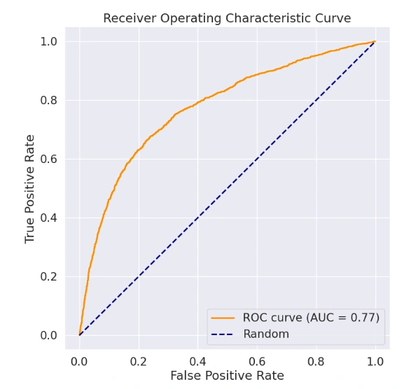
The below image shows the ROC Curve and ROC-AUC Score of the model:

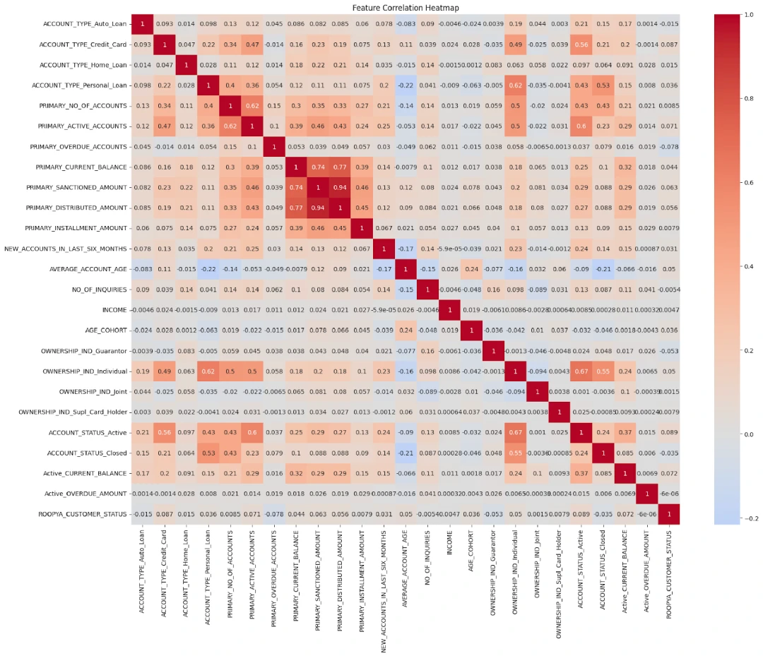
Sample Correlation Heat Map Between Variables:

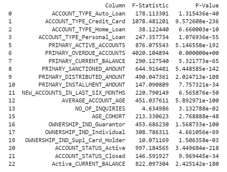
Sample p-values for each column and checked that these columns are significant for this model:

Here’s a table summarizing the performance metrics for the three models: Logistic Regression, Random Forest Classifier, and XGBoost Classifier.

Metric	Logistic Regression	Random Forest Classifier	XGBoost Classifier
Accuracy	0.7678	0.9665	0.9686
F1 Score	0.8608	0.9829	0.9840
AUC-ROC Score	0.8386	0.8169	0.8438
Gini Coefficient	0.6692	0.6337	0.6876
Precision	0.9896	0.9699	0.9699
Recall	0.7627	0.9964	0.9984
Specificity	0.7678	0.0476	0.0486

Final Scorecard Production

Creating a scorecard involves multiple steps, from initial data analysis to scaling and categorizing the scores.

Step 1: Initial Characteristic Analysis and Logistic Regression

Before producing the final scorecard, conduct initial characteristic analysis and logistic regression on the dataset to identify relevant characteristics and their coefficients.

Step 2: Scaling

Scaling refers to converting the logistic regression scores into a format that is more usable and understandable. The choice of scaling can vary depending on operational needs, regulatory requirements, and ease of interpretation. Some common scaling methods include:

Logarithmic Scaling: Score = Offset + Factor * ln(odds)

Factor and Offset can be calculated using simultaneous equations:

Score = Offset + Factor * ln(odds)

Score + pdo = Offset + Factor * ln(2 * odds)

Where:

Score:The credit score assigned to an applicant.
Factor:The scaling factor.
Offset:The offset value.
pdo:Points to double the odds (a specified value).
odds:The odds of default calculated from logistic regression.

Calculate Factor and Offset as follows:

Factor = pdo / ln(2)

Offset = Score – (Factor * ln(odds))

Credit Risk Modelling

Its Starts With Logistic Regression

Evaluation Metrics

Final Scorecard Production

Best In-class Features

COMPANY

SITEMAPS